The New Base Pipe
Here, we’re going to take a quick look at the new pipe introduced in the development version of R 4.1.0, and compare it to the well-known %>% pipe from the {magrittr} package that is used throughout the {tidyverse}.
There was a recent update to {magrittr} which switched to implementing the bulk of the piping in the C language rather than directly in R. Because of this, as well as showing some features of the new base pipe, |>, I’m going to compare it to both the new {magrittr} pipe, %>% and the old version, which I am going to style as %>>%
install.packages("magrittr")
remotes::install_github("Myko101/magrittrclassic")
If you want to install the classic {magrittr} without this updated %>>% pipe then run remotes::install_github("Myko101/magrittrclassic@classic") to have it loaded as a package called {magrittrclassic} or remotes::install_github("tidyverse/magrittr@v1.5) to have it overwrite your current {magrittr} package. Note that this is prone to errors, particularly if {magrittr} or any packages that depend on it are loaded.
The first thing to inspect is the speed of this new pipe in a simple situation. Let’s create a simple function and see how it goes in the bench::mark() function
doubler <- function(val) 2*val
x <- 1:10
bm <- bench::mark(
standard = doubler(x),
magrittrclassic = x %>>% doubler(),
magrittr = x %>% doubler(),
base = x |> doubler()
)
ggplot2::autoplot(bm)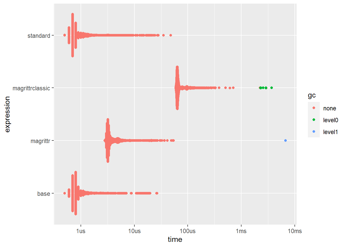 Note that the `bench::mark()`` function by default also checks whether the results we get are the same.
The first thing that jumps out is just how slow the old {magrittr} implementation is and how fast the base/standard versions are. The time scale on the plot is logarithmic, which shows that the old {magrittr} function is almost 2 orders of magnitude slower (800ns vs 72.5 us), that’s nearly 100x slower!
Why is this? Firstly, the old {magrittr} pipe builds functions in R and then applies them to data turn by turn. However, the new {magrittr} pipe does all this in C. How is the base version so much faster? Well it is a syntax rather than an infix operator or a call.
This means that x %>% f() builds functions and performs actions to produce output which is identical to f(x). However, x |> f() is the same as f(x), it’s just a different way of writing it. Think of using a single quote, ' or a double quote " to create a string, the command you’re giving to R is different, but the result is parsed identically before any actual R code is ran. Similarly, when you run 2 + 3 + 4, R will parse that as ( (2+3) + 4 )because the addition operator can only run on two objects so R has to divvy them up appropriately (left to right).
This can be evidenced by capturing the calls using the rlang::exprs() function
rlang::exprs(
  standard = doubler(x),
  magrittrclassic = x %>>% doubler(),
  magrittr = x %>% doubler(),
  base = x |> doubler()
)
## $standard
## doubler(x)
##
## $magrittrclassic
## x %>>% doubler()
##
## $magrittr
## x %>% doubler()
##
## $base
## doubler(x)See the last one there? x |> doubler() is exactly doubler(x). There’s no transforming in R here, it just is the same thing.
This functionality is added to by the introduction of a new lambda function creation shortcut, let’s compare it to the {magrittr} implementation(s) of anonymous functions, using the dot notation:
bm2 <- bench::mark(
  standard = (function(y) 2*y)(x),
  magrittrclassic = x %>>% {2*.},
  magrittr = x %>% {2*.},
  base = x |> \(y) 2*y
)
ggplot2::autoplot(bm2)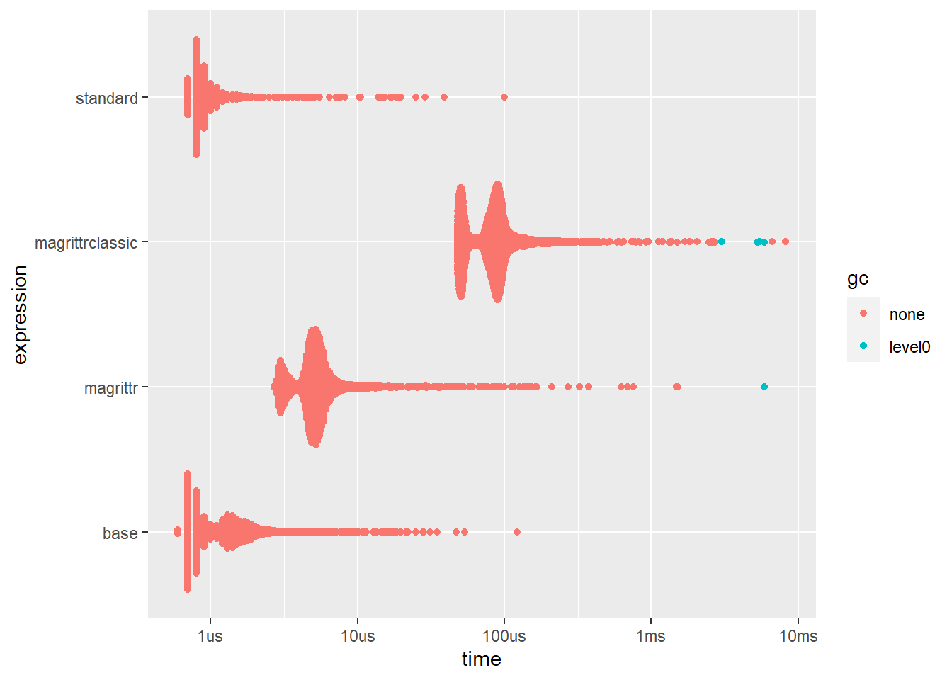
Timings are very similar to the previous one, especially when only looking relatively. The slow down is probably due to the creation of a function in each use, which also explains why they are all around the same amount slower. What do these piped lambda functions look like?
rlang::exprs(
  standard = (function(y) 2*y)(x),
  magrittrclassic = x %>>% {2*.},
  magrittr = x %>% {2*.},
  base = x |> \(y) 2*y
)
## $standard
## (function(y) 2 * y)(x)
##
## $magrittrclassic
## x %>>% {
## 2 * .
## }
##
## $magrittr
## x %>% {
## 2 * .
## }
##
## $base
## (function(y) 2 * y)(x)Again the standard and base versions are parsed the same.
One final critic of the new pipe is that you can only pass an object to the first argument in a function. This is a limitation in a lot of cases, particularly because most {base} functions don’t follow the convention of passing the current data as the first argument. In {magrittr}, we can use a . to represent the piped data for other arguments, and if it appears at the top level (i.e. a direct argument) {magrittr} won’t also ut it i as the first argument. But using the lambda \() syntax, we can get around this. We can also pass named arguments in the same way we usually would when calling a function. Let’s try it and time it
multiplier <- function(a,val) a*val
bm3 <- bench::mark(
standard = multiplier(2,x),
magrittrclassic = x %>>% multiplier(2,.),
magrittr = x %>% multiplier(2,.),
base_named = x |> multiplier(a=2),
base_lambda = x |> \(y) multiplier(2,y)
)
ggplot2::autoplot(bm3)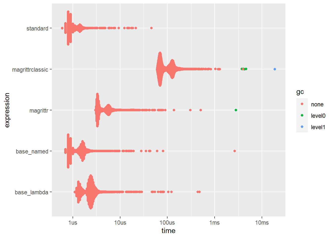 Clearly, the lambda version of the base packages takes more time, again because it is creating the function in the middle, whereas the named version does not have to do this. Let’s capture them to check that this is true
rlang::exprs(
  standard = multiplier(2,x),
  magrittrclassic = x %>>% multiplier(2,.),
  magrittr = x %>% multiplier(2,.),
  base_lambda = x |> \(y) multiplier(2,y),
  base_named = x |> multiplier(a=2)
)
## $standard
## multiplier(2, x)
##
## $magrittrclassic
## x %>>% multiplier(2, .)
##
## $magrittr
## x %>% multiplier(2, .)
##
## $base_lambda
## (function(y) multiplier(2, y))(x)
##
## $base_named
## multiplier(x, a = 2)One final thing to look at is the lambda function part of this whole process. While the {tidyverse} doesn’t provide a general shortcut to produce these, they can be created within other functions. For example, the above syntax {2*.} only works within the context of a pipe and wouldn’t work as a piece of code on it’s own.
The other major way in which lambda functions are declared is through the {purrr} package. The {purrr} package provides methods of functional programming (to an extent), and so within a {purrr} function, we can define a function using the ~ symbol and, like the previous {tidyverse} lambda, using the . as the value being passed to the function. Let’s compare it to the \() syntax, remember, this is again a syntax and not a function/call!
library(purrr,warn.conflicts=F)
bm4 <- bench::mark(
  standard = {
    res <- vector("list",10)
    for(i in 1:10) res[[i]] <- mean(1:i)
    res
  },
  purrr = map(1:10,~mean(1:.)),
  base = lapply(1:10,\(i) mean(1:i))
)
ggplot2::autoplot(bm4)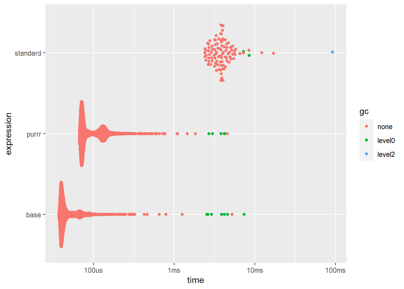
Again due to the lack of overheads for the \() syntax, speed is definitely on it’s side. We could just as easily use the lapply() function here and declare the FUN argument using function(i) mean(1:i), but writing \() is much quicker/easier.
One last thing to inspect is how these functions handle errors.
throw_error <- function(x){
  stop("OH NO!")
}
Previously, the trace stack for {magrittr} was confusing and made it incredibly difficult to spot where the error came from. Let’s see how
1:10 %>>%
  throw_error()
## Error in throw_error(.): OH NO!traceback()
# 10: stop("Why am I here?") at #2
# 9: throw_error(.)
# 8: function_list[[k]](value)
# 7: withVisible(function_list[[k]](value))
# 6: freduce(value, `_function_list`)
# 5: `_fseq`(`_lhs`)
# 4: eval(quote(`_fseq`(`_lhs`)), env, env)
# 3: eval(quote(`_fseq`(`_lhs`)), env, env)
# 2: withVisible(eval(quote(`_fseq`(`_lhs`)), env, env))
# 1: 1:10 %>>% throw_error()Because of the structure of the old {magrittr}, numbers 2 - 8 are functions that are called internally within the pipe and so as end-users, they mean nothing!
However, the new error handling, makes this much clearer without all the clutter:
1:10 %>%
  throw_error()
## Error in throw_error(.): OH NO!traceback()
# 3: stop("Why am I here?") at #2
# 2: throw_error(.)
# 1: 1:10 %>% throw_error()Now let’s compare to the base pipe:
1:10 |>
  throw_error()
## Error in throw_error(1:10): OH NO!traceback()
# 2: stop("Why am I here?") at #2
# 1: throw_error(1:10)The trace is even shorter. This is because in the {magrittr} pipe, the actual pipe is considered to be a call, and so it appears first in the trace stack (bottom of the list), BUT the base pipe is not a call, and so it doesn’t appear there at all. Just like when capturing the expression, the values are already nested.
Unlike errors though, warnings can be suppressed and code can continue, this means we can use the suppressWarnings() function to keep them quiet and just carry on. This is useful if you know about the warning beforehand, but is only recomended if you know exactly why the warning is appearing and just want your code to ignore it and run smoothly.
throw_warning <- function(x) {
  warning("oh no")
  x
}
This warning handling was one of the complaints about the old {magrittr} pipe,take the below which is instinctively what you would expect to do
1:10 %>>%
  throw_warning() %>>%
  suppressWarnings()
## Warning in throw_warning(.): oh no## [1] 1 2 3 4 5 6 7 8 9 10It doesn’t work, instead you’d have to run
suppressWarnings(
  1:10 %>>%
    throw_warning()
)
## [1] 1 2 3 4 5 6 7 8 9 10Which does not look pleasant and means going back to the beginning of your pipeline if you get to the point of wanting to suppress warnings.
The new {magrittr} pipe and the {base} pipe don’t have such qualms and they are evaluated exactly as you would expect them to:
1:10 %>%
  throw_warning() %>%
  suppressWarnings()
## [1] 1 2 3 4 5 6 7 8 9 101:10 |>
throw_warning() |>
suppressWarnings()## [1] 1 2 3 4 5 6 7 8 9 10